A Relative of ‘Siri’: The Voder

Image result for the voderImage result

While commuting between New York and New Jersey one evening, I tuned into the radio station 93.9 NYC as they started a technology portion of the show. The theme was language, and the first story was on using an translating app to navigate China (linked below), and the second was on this odd contraption called ‘the Voder’. Introduced at the 1939 World’s Fair, ‘The Voder’ was created by Homer Dudley and produced by the Bell Telephone Laboratory. This machine synthesized the first electrical human speech by producing the acoustic components of our speech. A woman ‘works’ the machine almost like a piano to control the various components of the Voder that allows it to ‘talk’. It  even sings “Auld Lang Syne” (a song that many of us today can’t even sing the lyrics to), which I find amazing, but at the same time creepy. Although this technology may seem dated compared to our ‘Siri’ and apps that can produce electronic language so fluidly and accurately, this was an important and interesting step forward in the realm of artificial language production. I wonder what amazing things we will invent today that will improve the communication and interaction of (or completely frighten) our children.

Listen to the story on ‘The Voder’ Here: http://www.wnyc.org/story/the-voder-the-first-machine-to-produce-human-speech/

Translation in Apps Story: http://www.wnyc.org/story/finding-a-pedicure-in-china-using-cutting-edge-translation-apps

Photo taken from : https://120years.net/the-voder-vocoderhomer-dudleyusa1940/


My Opinion: The Best and Worst Functions of Excel for this Project

spirited-away-successs

When creating our database, we had to input a large amount of information into each column for each index card. In this, I love the simple yet amazing ability to freeze the first row of the spreadsheet. Of course, the same can be done for columns.Whether we were on index card 2, 20, or 120, we could clearly see the column title of what type of information we were inputting.

Another function of excel that was awesome was the use of pivot tables. Pivot tables allowed us to quickly sort and count our data to give us an idea of  what our data would look like once uploaded for data visualization. For instance, with a pivot table we could see how many speakers were attributed to each language. We could also see who input what data, and sort by what type of information. For example, if one of the team member had clacked on my name, they could see how many cards I input were English. However, we decided not to keep it as part of our data set as the external visualization program we used allowed us to see the same information when we uploaded our data, even allowing clickable charts, maps, etc.

A final function that was greatly appreciated was the ability of an Excel spreadsheet to be uploaded onto Google drive, shared, then downloaded as an Excel file. This helped greatly, as the team felt most comfortable with Excel over the Google spreadsheet. Though I’m not sure if this should be attributed to Google or Microsoft (or both), this was none the less a great function.

But with the best, also comes the worst…

spirited-away-stairs-gif

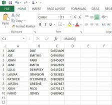
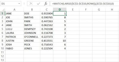
The biggest problem for me when starting this project was using qualitative data as opposed to quantitative data. When I had previously learned how to use an earlier version of Microsoft Excel early in high school, we worked with quantitative data and functions. In that, I found it a bit challenging in the beginning to just be putting in names and words instead of mathematical problems and functions.  However, I was surprised to find that when working in a column, excel will pop up with a cell fill-in for a word previously used. So say I was typing in the last name ‘Smith’ for a second or fifth time, I would have only typed up to the ‘m’ and excel would suggest “Smith” to put into the cell.

excel-fill-in-part-2

Where this turns sour for me is that if you skip a cell down and start typing into the second cell underneath, it no longer has the fill in as an option. I REALLY wish that this carried over while in the same column. When it came to really long or odd names, I really wished that excel would still automatically suggest a word fill in, even when you skip the cell of the next row. excel-fill-in-part-3

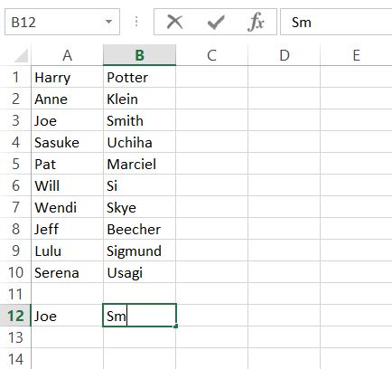
When trying to visualize our data, we ran into a problem. Where we had input  just countries or regions (i.e. Atlantic Midland, Inland North, etc.) as the language’s origin, the visualization technology we were using could not figure out how to map the languages with just the country. In that, we had to go back and put in the capital of each country of the languages origin, and designate a ‘capital’ for different types of English (i.e. North Jersey vs. South Jersey English), which resulted in a more accurate depiction of the locations of each language origin. Overall, I wish that Microsoft Excel would improve on it’s compatibility with other software and websites. Though I understand there’s much time, thought, and agreement that needs to be done for this, companies like Amazon and Paypal work with other websites and services to create a smoother use of services. Therefore, Microsoft does have the ability to work better with other companies’ programs, and I wish that both parties would work to do so in the near future.


Both of the above images do not belong to me. ‘Spirited Away’ is the property of Studio Ghibli/Disney and were found here: giphy.com/search/spirited-away-gif

How Do You Say…’Hello’?

In gathering our data, we have recorded many different languages. Here is how you say hello in some of them!

English ~ Hello/Hi

Italian ~ Ciao

German ~ Hallo

French ~ Bonjour

Tagalog ~ Kamusta

Spanish ~ Hola

Russian ~ Здравствуй   (Zdravstvuy) 

Welch ~ Helo

Dutch ~ Hoi

Japanese ~ こんにちは  (Kon’nichiwa)

Korean ~안녕   (annyeong)

Polish ~  cześć

Gaelic ~ Haigh

Portuguese ~ Oi

Chinese (Cantonese/Mandarin) ~  你好  Nǐ hǎo

greeting-2

Microsoft Excel: Randomized Number I.D. for Participants

In order to present our data by the participant, the ethical thing was to avoid revealing the actual name of the individuals who gave us our data. In this, we used Microsoft Excel to generate and assign random numbers, rather than simply numbering every subject individually. These numbers would then act as the I.D.’s for each participant. On a separate spreadsheet, we put participants first and last names in columns ‘A’ and ‘B’ respectively (here I have put in ten fake names* to show you an example). For our data, we had a list of all the participants’ names in alphabetical order by last name.

random-number-excel-part-3

Next, I used the RAND, or random function. By putting the =RAND() function into column ‘C’ from cells C1 to C10, we were given a random decimal number. Then, I had tried to use the =RANDBETWEEN function in column ‘D’, inputting =RANDBETWEEN(1,10). Although this gave us a random whole number between 1 and 10, there were repeats of the same number. So now one of the biggest problems was finding a way to have excel create random intergers that did NOT repeat.

random-number-excel-part-2

Finally, with a little help from the library and the internet, I used the following formula to generate NON-REPEATING whole numbers in column ‘D’;
=MATCH(LARGE($C$1:$C$20,ROW()),$C$1:$C$20,0)


The result was what we were looking for, anonymity for our participants. With this success, we copied and pasted the numbers next to the names in the list of participants in our data set.**

random-number-excel-part-1

*None of these names are meant to have any relation to any person(s) alive or deceased.
**When I input the function into column ‘D’, the random values in column ‘C’ changed automatically, but remained random. you need to keep this formula in this column in order for the function in ‘D’ to work.


There may be other ways of achieving the same outcome, but this formula worked best in excel.

Microsoft Excel vs. Google Sheets: Which One Did We Choose?

Initially, we were going to use Google’s spreadsheet because we could all edit it in one place, but we encountered a few problems. Some of the data in the Microsoft Excel spreadsheet when opened in the Google spreadsheet would overlap into other columns, making it hard to read. Additionally, there would be the occasion where data that was present in the Excel sheet was missing in Google’s spreadsheet. As another point, we all had the same version (2013) of Microsoft Excel  pre-downloaded on our laptops which made Microsoft Excel compatibility easy. It was unanimously decided that we use Microsoft Excel to input data. However, we also decided to use Google Drive to save and share our data on a cloud. Google Drive also updated us via email anytime one of us contributed to our shared folder.

We created three folders in google docs to organize our saved spreadsheets and other files. These three were ‘1st DH Raw Data’, ‘2nd DH Raw Data’, and ‘DH Meeting Docs’. The third folder held our meeting minutes, or what our discussions were when we met and what goals we discussed to have done before we next met. Both the first and second raw data folders had sub folders of ‘checked’ and ‘unchecked’, where the previously naming convention came in handy. Additionally, both raw data set folders had their respective index card scanned copies were saved there. In doing this, we kept all files organized well and were able to share files efficiently. Although we all saved the most recent files to our desktops and to a shared USB drive for backup, Google Drive assured that our updated and previous files were in one place that we could all access from any computer.

Our Naming Convention and Communication

All data we entered had to not only be divided evenly among the team, but it also needed to be checked to make sure that the information is correct and who had last saved the data. We agreed to use an author naming convention by using our initials. In the Microsoft Excel spreadsheets, we designated four additional columns for this purpose, and two more columns were added to communicate on the spreadsheet itself. Columns D,E, R, S, T, and U were used for the following: D was ‘Entered by CQ/MP/AB/EH’, E was ‘Date Entered’, R was ‘Comments’, S was ‘Checked by CQ/MP/AB/EH’, T was ‘Date Checked’, and U was ‘Additional Notes’.  The ‘Comments’ column was used to communicate changes to data. Say I had entered a name wrong as ‘McThomas’, but Michelle caught the mistake, and would write in that row under column R ‘MP-AB fixed last name to MacThomas’. This tells us that Michelle is writing to Anastasia (me) that she fixed the error in the last name I made. If we had a question or were not sure of a data entry or part of one, we would write in column R as well. For example, if Ellie had a question about  a missing name, she could write in the ‘Comments’ column ‘Which participant is this?’ or simply state ‘No name given’.

The initial convention was used not only to show who input and checked the data, but also who had last saved the data. To give an example, if I was the first to put in data, I would label the newly saved excel sheet ‘AB Raw Data Set 1’.  If Ellie was the next to input her data and check mine, the new excel sheet would be titled and saved as ‘AB-EH Raw Data Set 1’. Then, if Michelle were to do the same, the file would be saved as ‘AB-EH-MP Raw Data Set 1’. This naming method would continue until all data is input and checked.

Overall, this system of using our initials to know who last saved, checked, and input data worked very well. It was a simple, clear way to know among the team who had last saved the most recent data and who was communicating with who within the spreadsheet, especially between meetings.